
The Hidden Geometry of Transformer Weights:
A Canonical Basis for Interpreting Transformer Language Models
Abstract
We report the discovery of a hidden geometric structure inside Transformer language models, visible after rotating the model into a coordinate system aligned with its own weight matrices — the canonical basis. In this basis, the 896-dimensional hidden space of Qwen 2.5 0.5B reveals: a bipolar oscillator that rhythmically alternates between knowledge-receptive and filtering modes across layers — the model's respiration; a homeostatic mechanism that erases any intermediate perturbation within two layers; a spectral collapse wherein singular value magnitudes are redundant across layers; and a correlation-based knowledge representation where facts are encoded in patterns of co-activation rather than on individual axes.
Version 2 adds the causal evidence and the architectural generality. The canonical-basis realignment is lossless, verified on three architectures: Qwen 2.5 0.5B (PPL 25.38 = 25.38, MMLU 47.50% = 47.50%), SmolLM2 1.7B (PPL 6.6018 → 6.6045, top-5 overlap 5/5), and — via a DC-preserving rotation that keeps LayerNorm untouched — Pythia 1.4B (PPL 9.2286 → 9.2359, greedy generation identical on 3/3 prompts).
The geometric structure is functional, not decorative. Zeroing a single canonical axis — axis 62, 0.11% of the model — collapses MMLU from 47.50% to 21.25% (−26.25 percentage points) and destroys output coherence (PPL 4.24 → 23858). Zeroing its anti-correlated partner axis 570 degrades factual accuracy while preserving fluency. Five control axes show no effect (≤ ±1.25 pp).
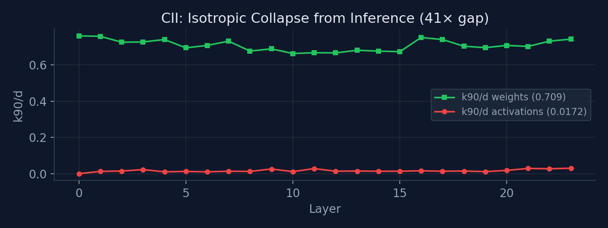
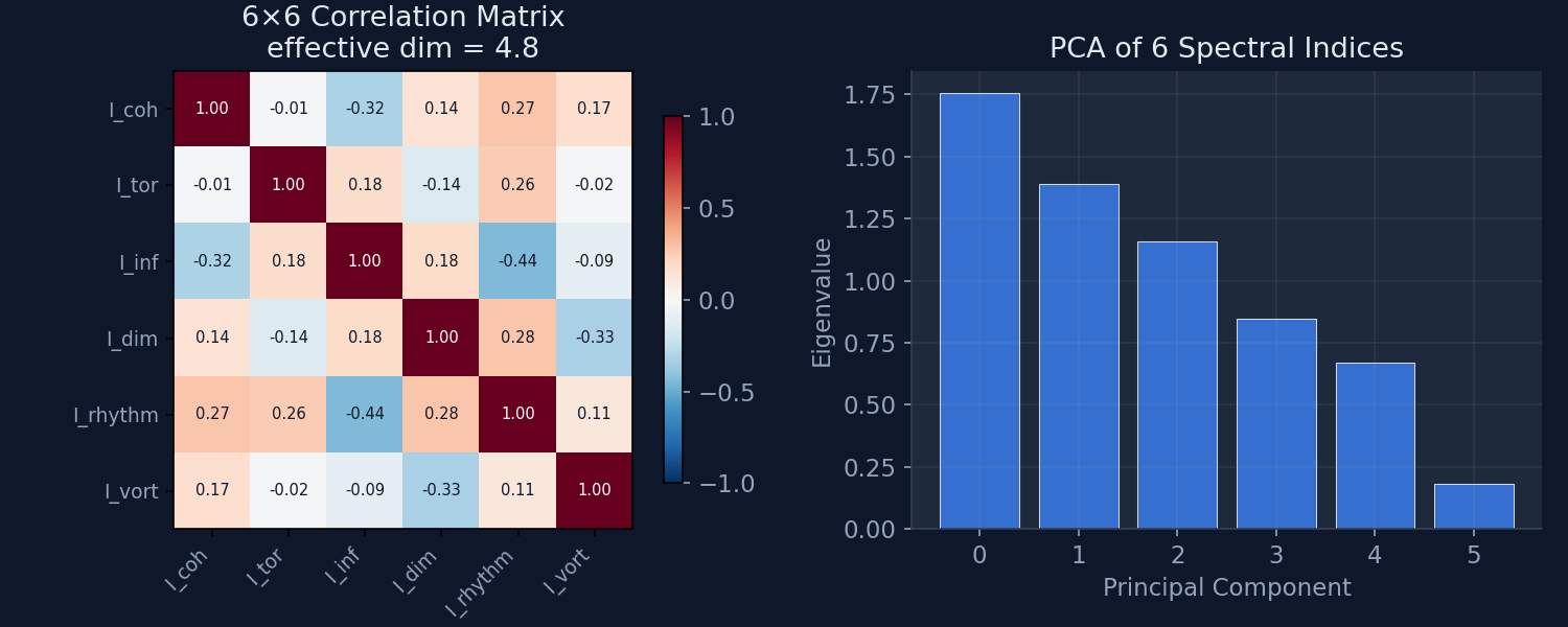
Six per-layer spectral indices quantify the structure (means 0.588 / 0.917 / 0.709 / 0.378 / 0.595 / 0.650) with effective dimensionality 4.77 out of 6, and expose a 41× isotropic collapse between the weight spectrum (k90/d 0.71) and the activation spectrum (k90/d 0.017).
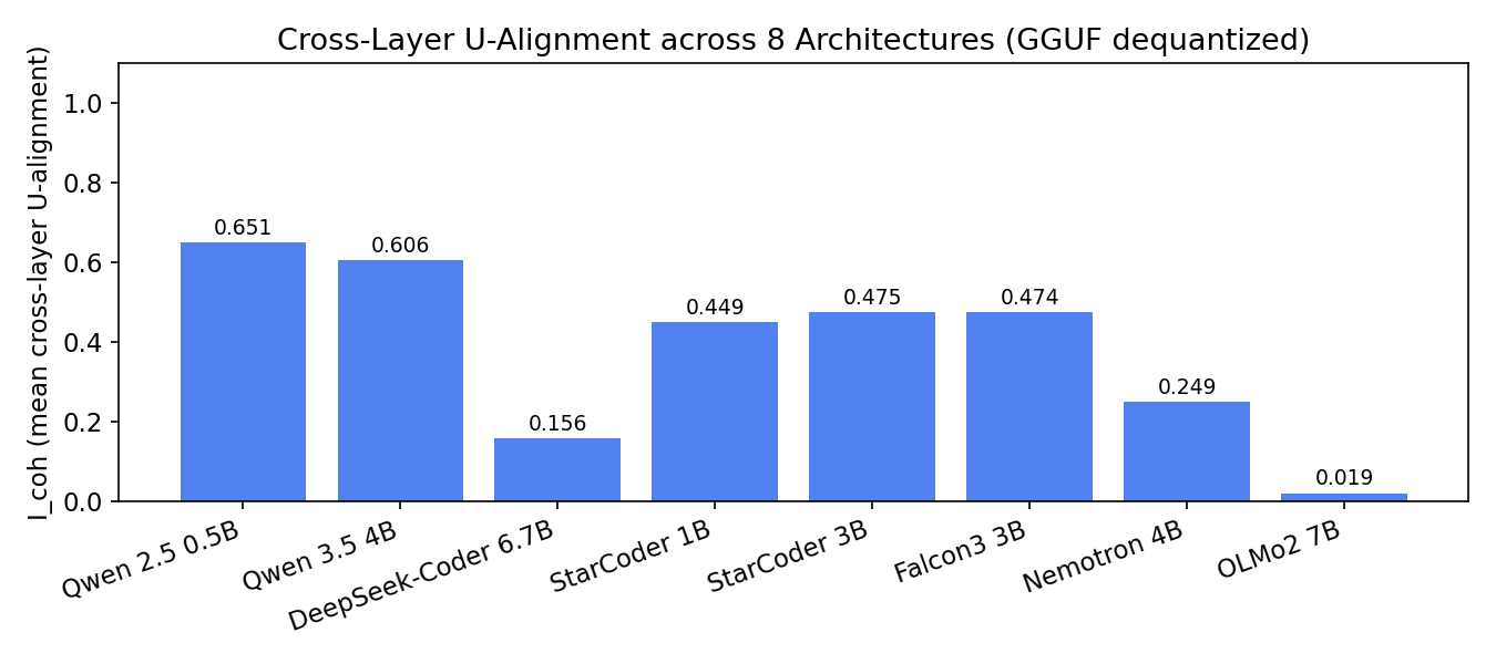
Native cross-layer U-alignment of the FFN writer, measured with one consistent method across eight architectures: Qwen 2.5 0.5B 0.651, Qwen 3.5 4B 0.606, Falcon3 0.474, StarCoder 0.475, Nemotron 0.249, DeepSeek-Coder 0.157, OLMo2 0.020. On the OLMoE-1B-7B MoE model (64 experts), per-expert cross-layer alignment is 0.086 and cross-expert alignment is 0.111.
1. Introduction
Version 1 of this work (Gernone 2026) posed a question: what happens if we rotate a Transformer language model so that the coordinate axes align with the directions the model itself considers important? It established the canonical basis — a lossless rotation built from the model's own singular vectors — and described five phenomena visible only in that basis: the bipolar oscillator (rich club), the layer-phased respiration, homeostasis, the spectral collapse, and correlation-based knowledge. Version 1 verified the realignment's losslessness on Qwen 2.5 0.5B.
Version 2 does three things. First, it answers the question version 1 left open: is the observed structure functional, or merely decorative? Section 5 provides the causal test — single-axis ablation. Second, it turns the qualitative descriptions into a quantitative instrument: the six spectral indices (Section 4). Third, it tests how far the framework generalizes: two additional realignments (SmolLM2, Pythia), eight architectures measured for native alignment, and a MoE model (Section 6).
One correction is in order. Version 1's experimental table attributed a mean cross-layer U-alignment of 0.944 (max 0.991) to Qwen 2.5 0.5B. That value was measured on Qwen 3.5 4B (33 layers, 528 pairs) with a different pipeline, and was carried into version 1's table by mistake. Measured with the single consistent method used throughout this version, native Qwen 2.5 0.5B shows 0.651 (max 0.928, all 276 pairs) — still far above the random baseline of 0.027 for d=896. The corrected table is in Section 6.3.
2. The Method: Canonical Basis for Language Models (CBLL)
A Transformer's internal state is a vector in R^d — the residual stream. Everything the model knows passes through this space, but the basis in which it lives is arbitrary — whatever the training converged to. The canonical basis rotates the model so that axis k of the hidden state corresponds to a specific spectral direction of the model's own weight matrices.
2.1 RMSNorm architectures (established in version 1)
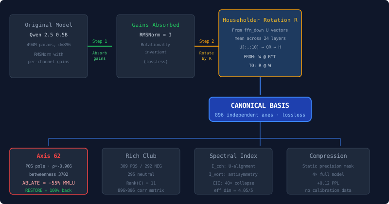
1. Absorb RMSNorm gains. Fold the per-channel gain g of each RMSNorm into the adjacent weight matrix columns: W' = W @ diag(g). All RMSNorm gains become 1.0; the normalization commutes with any orthogonal rotation.
2. Build the rotation. Average the top-K left singular vectors of ffn_down across layers, orthonormalize, complete to a full orthogonal matrix R with Householder reflectors.
3. Apply. FROM-d_model matrices rotate with W @ R^T (q, k, v, gate, up); TO-d_model matrices with R @ W (o_proj, down_proj). Hooks rotate the embedding output (embed @ R^T) and un-rotate the last layer output (hidden @ R).
The transformation is functionally lossless — verified in version 1 and again in Section 6.
2.2 LayerNorm architectures (new in version 2)
LayerNorm subtracts the mean: LN(x) = (x − μ)/σ ⊙ γ + β. The mean subtraction is equivariant under rotation iff the rotation fixes the ones-vector:
μ(h R^T) = (1/d) · h R^T 𝟙 = (1/d) · h 𝟙 = μ(h) ⟺ R^T 𝟙 = 𝟙
Therefore LayerNorm models admit the canonical basis under a DC-preserving rotation — a rotation whose invariant direction is 𝟙/√d. The procedure:
1. Absorb γ and β. γ into FROM weight columns (W' = W @ diag(γ)), β into FROM projection biases (b' = b + W_orig @ β). Exact, because the absorption is followed by a linear projection.
2. Build a DC-preserving rotation. Householder reflectors H = I − 2uu^T with u ⊥ 𝟙, each fixing the ones-vector; the product fixes it too.
3. Apply. FROM = W @ R^T, TO = R @ W, and TO biases as b @ R^T — critical for bias-carrying architectures. Qwen-class models have no biases; GPT-NeoX has biases on every projection.
4. Hooks as in 2.1. LayerNorm remains untouched, becoming pure centering (x − μ)/σ, which commutes with the DC-preserving rotation.
Verified lossless on Pythia 1.4B (Section 6.2).
3. Established Findings (version 1, summarized)
Version 1 established five phenomena in the canonical basis of Qwen 2.5 0.5B. They are summarized here for completeness.
3.1 The Rich Club and the Bipolar Oscillator
The dominant eigenvector of the 896 × 896 activation correlation matrix divides the axes into two poles:
| Property | Positive Pole | Negative Pole |
|---|---|---|
| Axes | 309 | 292 |
| Top axes | [9, 262, 62, 8, 629] | [2, 6, 570, 4, 207] |
| Mean energy | 0.250 | 0.260 |
Of the 309 positive-pole axes, 83% possess a dedicated inhibitory partner in the negative pole — an axis with which they are strongly anti-correlated. The master pair, axis 62 ↔ axis 570, has ρ = −0.97: when one fires, the other is silenced. The effective rank of the correlation matrix is 11 — only eleven independent correlation patterns exist in the entire model.
3.2 Respiration — Layer-Level Bipolar Control
The POS/NEG activation ratio oscillates across the 24 layers in four phases, invariant to input content:
| Phase | Layers | POS/NEG Ratio | Interpretation |
|---|---|---|---|
| Encode | 0–4 | 1.36 | POS dominant — the model receives information |
| Process | 5–20 | 0.42–0.88 | NEG dominant — the model filters and selects |
| Decode | 21 | 1.28 | POS peak — the model prepares the response |
| Output | 23 | 0.54 | NEG dominant — filtered output emitted |
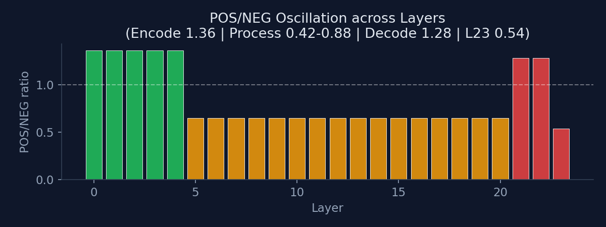
The same five layers — [21, 3, 23, 2, 22] — are the top activators for every prompt tested. The respiration is not a response to the content. It is a structural signature of the model's operation.
3.3 Homeostasis: Why You Cannot Push the Residual Stream
A multiplicative gain applied to a specific canonical axis at the output of a specific layer:
Gain 5× applied to axis a at layer 0:
  Layer 0:  5.0×  ← the amplification works locally
  Layer 1:  1.4×  ← already diluted
  Layer 2:  1.0×  ← completely erased
  Layers 3–23: 1.0×  ← no trace remains
The residual stream is homeostatic: any perturbation of the intermediate activations is annulled within two layers, by the combined action of RMSNorm re-normalization, attention softmax saturation, and the SiLU operating range. The two-layer decay constant is invariant to injection position — the same decay curves appear when the gain is injected at layers 5, 12 and 21.
The consequence is that you cannot steer the model by injecting signals into the intermediate layers. The model will erase the intervention. The only way to modify the behaviour is to modify the weights — the transformations themselves — rather than the signals that flow through them.
3.4 Spectral Collapse: S is Redundant
The feed-forward hidden states form a 3-tensor H ∈ R^{L × N × d}. A Tucker decomposition reveals the cross-layer structure: the geometric rank (U) is 22 of 24 layers — the directions of the singular vectors vary independently across layers; the spectral rank (S) is 1 of 24 layers — the magnitudes of the singular values are almost identical across all layers, with a single vector explaining 90% of the cross-layer variance (first-to-second ratio 23.2×). When the singular values are replaced with randomly shuffled values and the model is reconstructed, it still produces coherent text. The model operates on geometry, not on intensity.
3.5 Knowledge is in Correlations, Not in Axes
The axes with the highest per-axis entropy — 268 "knowledge carriers", the most structured activation patterns — overlap almost entirely (241/268) with already active axes. Knowledge is not stored in dedicated axes; it is distributed. The effective rank of the correlation matrix is 11: the model's entire knowledge structure — facts, reasoning, language, style — can be described by 11 independent correlation patterns across 896 axes. Facts are encoded in patterns of co-activation between axes, not in individual axis values. Individual axes are letters; the correlation structure is the language.
4. The Six Spectral Indices (new in version 2)
To turn the qualitative observations into a quantitative instrument, version 2 defines six per-layer spectral indices (data: data/six_indices_entropy.json):
| Index | Name | What it measures | Mean ± std |
|---|---|---|---|
| I_coh | Cohesive | Cross-layer U-alignment (top-20 left singular vectors of ffn_down, adjacent layers) | 0.588 ± 0.112 |
| I_tor | Torsional | V-rigidity across adjacent layers | 0.917 ± 0.002 |
| I_inf | Informational | Spectral flatness of the weights (k90/d of ffn_down) | 0.709 ± 0.030 |
| I_dim | Dimensional | Effective rank of the activations (PCA k90/d per layer) | 0.378 ± 0.053 |
| I_rhythm | Rhythmic | Cosine similarity between layer input and layer output | 0.595 ± 0.147 |
| I_vort | Vorticity | Activation antisymmetry A(C) of C = E[h ⊗ ffn_out^T] | 0.650 ± 0.130 |
Three properties make these indices a measurement framework:
Near-independence. The correlation matrix of the six indices has effective dimensionality 4.77 out of 6. The dominant correlation direction loads positively on I_rhythm (+0.685) and I_dim (+0.469), negatively on I_coh (−0.516).
Divergent variance profiles. I_tor is essentially constant across layers (std 0.002). I_coh and I_rhythm vary widely, tracing the respiration phases. I_vort shows two collapses — L3 (A = 0.176) and L21 (A = 0.293) — and maximum torsion at L22 (A = 0.707) before output.
The isotropic collapse from inference. The weights carry a flat spectrum (I_inf = 0.709), but activations during inference are nearly one-dimensional (global k90/d of pooled activations 0.017) — a 41× gap. Stronger cross-layer U-alignment correlates with less orthogonality bending of the activation cross-correlation (r = −0.442, data: data/magnetism_magnitude_bending.json).
5. Causal Evidence: Single-Axis Ablation (new in version 2)
Descriptive structure can be dismissed as decorative. The causal test: remove a single axis and measure what breaks.
Method. Output axis k of the FFN is controlled by row k of W_down in every layer (ffn_out[:, k] = Σ_i intermediate[:, i] · W_down[k, i]). Zeroing row k in all 24 layers removes the FFN's contribution to axis k — a weight-level intervention, immune to homeostasis.
Protocol. Qwen 2.5 0.5B Instruct, canonical basis. MMLU 12 subjects × 20 questions (240 total). Baseline 47.50% (114/240). Nine axes tested. (Data: data/single_axis_ablation.json; script: scripts/ablate_single_axis.py.)
| Axis | Role | MMLU | Δ (pp) | PPL | Δ PPL |
|---|---|---|---|---|---|
| 62 | Rich Club hub, betweenness 3702 | 21.25% | −26.25 | 23858 | +23854 |
| 0 | First canonical axis | 37.92% | −9.58 | 228.7 | +224.4 |
| 570 | Anti-correlated partner of 62 (ρ=−0.97) | 44.58% | −2.92 | 4.29 | +0.05 |
| 400 | Empty/low-energy axis | 44.58% | −2.92 | 4.33 | +0.09 |
| 50 | Control | 48.75% | +1.25 | 4.29 | +0.05 |
| 100 | Control | 48.75% | +1.25 | 4.23 | −0.01 |
| 200 | Control | 46.67% | −0.83 | 4.16 | −0.08 |
| 500 | Control | 47.50% | 0.00 | 4.19 | −0.05 |
| 800 | Control | 47.92% | +0.42 | 4.55 | +0.31 |
Qualitative outputs. With axis 62 zeroed, chat generation produces unstructured token fragments. With axis 570 zeroed, generation remains syntactically fluent but factually wrong — "What is the capital of Italy?" yields "Florence" where the baseline yields "Rome". Knowledge and fluency live on different axes.
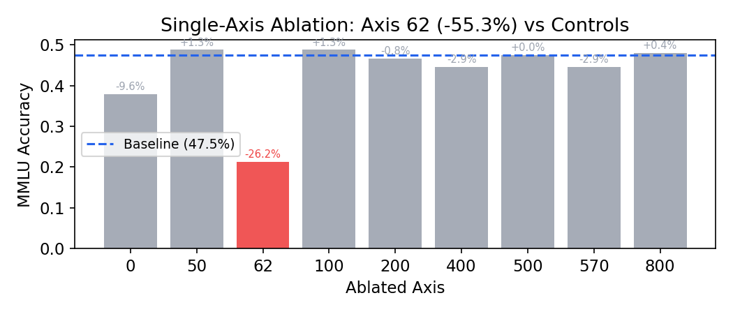
Interpretation. One axis out of 896 (0.11%) destroys the model. Five control axes do nothing. The geometric structure is causal, not decorative.
Interactive reproduction. demo/chat.py ships with the repository: a per-axis control chat that realigns the model on first run, then zeroes and restores any axis mid-conversation (/ablate 62, /restore). The effect is immediate and reversible.
Cross-family replication. On SmolLM2 1.7B, zeroing canonical axis 0 at the last layer raises PPL from 6.60 to 3874; axes 50–2047 change PPL by ≤ 0.10 (data: data/smollm_cbll_access_indices.json).
6. Multi-Architecture Verification (new in version 2)
All experiments in this section use the method of Section 2. Hardware: NVIDIA GTX 1660 Ti 6 GB, fp16 inference, fp32 algebra.
6.1 Realignment Losslessness
| Model | Metric | Original | Realigned | Δ |
|---|---|---|---|---|
| Qwen 2.5 0.5B | MMLU (12 subjects) | 47.50% | 47.50% | 0 |
| Qwen 2.5 0.5B | MMLU Pro | 15.50% | 15.50% | 0 |
| Qwen 2.5 0.5B | WikiText PPL | 25.38 | 25.38 | 0 |
| SmolLM2 1.7B | WikiText PPL | 6.6018 | 6.6045 | +0.0026 |
| SmolLM2 1.7B | Max logit diff (4 prompts) | — | 3.9–7.0 × 10⁻² | fp16 noise |
| SmolLM2 1.7B | Top-5 overlap | — | 5/5 | — |
| Pythia 1.4B (LayerNorm, DC bridge) | WikiText PPL | 9.2286 | 9.2359 | +0.0073 |
| Pythia 1.4B | Greedy generation | — | 3/3 identical | — |
6.2 The LayerNorm Bridge — DC-Preserving Rotation
LayerNorm is rotation-equivariant iff the rotation fixes the ones-vector. The lossless bridge keeps LayerNorm and rotates with a DC-preserving matrix. Data: data/pythia_dc_bridge_results.json, script: scripts/pythia_dc_bridge.py. On Pythia, canonical-basis access is verified: zeroing axis 1 raises PPL by 0.62; axes 0/500/1000/2047 change PPL by ≤ 0.07. U-alignment in the canonical basis is 0.397 (max 0.958); k90/d is 0.715.
6.3 Native Alignment across Eight Architectures
Native cross-layer U-alignment of the FFN writer, measured with one consistent method (dequantized weights, top-1 left singular vector, all layer pairs). Script: scripts/analyze_gguf_cbll.py, data: data/gguf_cbll_multiarch.json:
| Model | Normalization | U-alignment (mean) | Max | k90/d |
|---|---|---|---|---|
| Qwen 2.5 0.5B | RMSNorm | 0.651 | 0.928 | 0.760 |
| Qwen 3.5 4B | RMSNorm (hybrid Mamba-FFN) | 0.606 | 0.926 | 0.706 |
| Falcon3 3B | LayerNorm | 0.474 | 0.950 | 0.670 |
| StarCoder 3B | LayerNorm | 0.475 | 0.970 | 0.664 |
| StarCoder 1B | LayerNorm | 0.449 | 0.951 | 0.668 |
| Nemotron-Mini 4B | RMSNorm + bias | 0.249 | 0.923 | 0.660 |
| DeepSeek-Coder 6.7B | RMSNorm | 0.157 | 0.848 | 0.583 |
| OLMo2 7B | non-parametric LayerNorm | 0.020 | 0.477 | 0.677 |
Alignment strength varies widely. Normalization type alone does not determine it: LayerNorm models can align (Falcon3, StarCoder: 0.45–0.47), RMSNorm models can fail to (DeepSeek: 0.16), and normalization without learnable parameters produces random alignment (OLMo2: 0.020, random baseline ≈ 0.013 for d=4096).
6.4 MoE: OLMoE-1B-7B
OLMoE (16 layers, 64 experts, top-8 active, RMSNorm) was realigned losslessly (rotated fp16 weights verified bit-level against PyTorch in a C inference engine). Spectral analysis of the rotated weights (script: scripts/analyze_olmoe_cbll.py, data: data/olmoe_cbll_summary.json):
| Measurement | Value |
|---|---|
| Dense o_proj U-alignment (mean/max) | 0.295 / 0.933 |
| Per-expert cross-layer U-alignment (down_proj) | 0.086 ± 0.097 |
| Cross-expert same-layer U-alignment (L8) | 0.111 (max 0.741) |
| k90/d dense o_proj (full SVD) | 0.447 |
| k90/d expert down_proj (full SVD) | 0.316 |
| Sigma cross-layer rank90 (expert 0) | 2/16, adjacent cos 0.9965 |
The expert structure is per-expert: experts do not share output directions across layers the way dense FFNs do. Cross-layer sigma redundancy (adjacent cos 0.9965) extends to the MoE setting.
7. Reproducibility
Every measurement in this paper is backed by a script and pre-computed data in the repository:
| Claim | Script | Data |
|---|---|---|
| Realignment (Qwen, SmolLM2, Pythia) | save_model.py, realign_smollm_cbll.py, pythia_dc_bridge.py | data/ |
| Cross-layer alignment | diagnose_shared_sigma.py | shared_sigma_diagnosis.json |
| Rich Club / respiration | investigate_rich_club.py | rich_club_investigation.json, respiration_data.json |
| Correlation structure | analyze_correlations.py | correlation_analysis.json |
| Six spectral indices | CBLL compendium tests | six_indices_entropy.json, magnetism_magnitude_bending.json, activation_antisymmetry.json |
| Spectral collapse | measure_6d.py | ten6or_measurement.json |
| Single-axis ablation | ablate_single_axis.py | single_axis_ablation.json |
| SmolLM2 access | smollm_cbll_continue.py | smollm_cbll_access_indices.json |
| Multi-architecture table | analyze_gguf_cbll.py | gguf_cbll_multiarch.json |
| OLMoE MoE analysis | analyze_olmoe_cbll.py | olmoe_cbll_summary.json |
| Pythia DC bridge | pythia_dc_bridge.py | pythia_dc_bridge_results.json |
Full reproduction from a clean Qwen checkpoint: bash reproduce.sh (6 steps, ~30 minutes on a 6 GB GPU). The repository is at github.com/todotge/canonical-basis.
8. Related Work
Mechanistic interpretability (Bricken et al. 2023; Templeton et al. 2024; Elhage et al. 2021) identifies individual features and circuits using sparse autoencoders. These approaches analyze what activates for which inputs. Our work analyzes the global geometric structure that underlies all activations.
Cross-layer weight continuity (Jeong, Paeng & Suh 2026, arXiv:2605.04971) independently observes that principal singular vectors of adjacent layers align ("geometric continuity") and attributes it to residual connections and symmetry-breaking. Our measurements extend the observation across eight architectures, add the canonical-basis transformation, and provide the causal ablation.
Activation engineering (Turner et al. 2023; Zou et al. 2023) adds steering vectors to model activations. The homeostasis finding suggests these vectors are partially erased within two layers, which may explain their variable effectiveness.
Weight matrix decomposition (Hsu et al. 2022) uses SVD for model compression. We confirm direct SVD compression is limited by the relatively flat spectrum of feed-forward layers (k90/d ≈ 0.76), and show the model's information is in the geometry (U subspace), not the spectrum (S vector).
Model merging and rebasin (Ainsworth et al. 2023; Singh & Jaggi 2020) aligns models using permutation symmetries. Our realignment uses continuous rotation, not discrete permutation, and exploits the structure within a single model rather than between models.
9. Limitations
The causal ablation and activation-level analyses are fully mapped on Qwen 2.5 0.5B; realignment losslessness is verified on Qwen 2.5 0.5B, SmolLM2 1.7B, and Pythia 1.4B (via the DC bridge). The multi-architecture alignment table uses GGUF-quantized weights (dequantized before SVD); top singular vectors are robust to quantization noise, and Qwen 2.5 0.5B was additionally measured on native HuggingFace weights with the same method (0.651, matching the GGUF-consistent pipeline within 0.3%).
The realignment requires full-precision (fp32) rotation matrices. fp16 forward passes introduce logit differences on the order of 10⁻² — behaviorally invisible (top-5 5/5, greedy generation identical) but not bit-exact.
Respiration and rich-club membership on models beyond 1.7B remain to be mapped; the OLMoE analysis is weight-level only.
The interpretation of the bipolar oscillator as "respiration" is a functional metaphor. The precise computational role of each pole — what the positive-pole axes do compared to what the negative-pole axes do — still needs to be characterized through ablation studies.
10. Conclusion
Rotating a Transformer language model into a coordinate system aligned with its own weight matrices reveals a hidden internal structure. Version 1 established the phenomena; version 2 establishes that they are functional and general:
1. A bipolar oscillator — 309 positive-pole and 292 negative-pole axes in rhythmic alternation across layers, invariant to input content.
2. A homeostatic mechanism — the residual stream erases any intermediate perturbation within two layers.
3. Spectral redundancy — singular value magnitudes are nearly identical across layers; the model operates on geometry, not intensity.
4. A six-index measurement framework — cohesive, torsional, informational, dimensional, rhythmic, and vorticity indices quantify the structure per layer with effective dimensionality 4.77/6, exposing the 41× isotropic collapse between weight and activation spectra.
5. Correlation-based knowledge — facts are encoded in patterns of co-activation; effective rank 11.
6. Causal structure — zeroing a single axis (62, 0.11% of parameters) collapses MMLU by 26.25 pp and destroys coherence; control axes show no effect.
7. Architectural generality — the realignment is lossless on RMSNorm and LayerNorm architectures; native alignment strength varies by family (0.02–0.65) and is not determined by normalization type alone.
The black box has geometry. You just need to look from the right angle.
Acknowledgments
We thank the open-source community for the models, datasets, and tools used in this research: Qwen, SmolLM2, Pythia, OLMoE, StarCoder, Falcon3, Nemotron, OLMo2, DeepSeek-Coder; the GGUF ecosystem; HuggingFace.
References
1. Bricken, T. et al. (2023). Towards Monosemanticity: Decomposing Language Models With Dictionary Learning. Anthropic.
2. Templeton, A. et al. (2024). Scaling Monosemanticity: Extracting Interpretable Features from Claude 3 Sonnet. Anthropic.
3. Turner, A. M. et al. (2023). Activation Addition: Steering Language Models Without Optimization. arXiv:2308.10248.
4. Zou, A. et al. (2023). Representation Engineering: A Top-Down Approach to AI Transparency. arXiv:2310.01405.
5. Hsu, Y.-C. et al. (2022). Extreme Compression of Large Language Models via Low-Rank Approximation. NeurIPS.
6. Ainsworth, S. K. et al. (2023). Git Re-Basin: Merging Models modulo Permutation Symmetries. ICLR.
7. Singh, S. P. & Jaggi, M. (2020). Model Fusion via Optimal Transport. NeurIPS.
8. Elhage, N. et al. (2021). A Mathematical Framework for Transformer Circuits. Anthropic.
9. Park, K. et al. (2024). The Geometry of Categorical and Hierarchical Concepts in Large Language Models. arXiv.
10. Marks, S. & Tegmark, M. (2023). The Geometry of Truth: Emergent Linear Structure in LLM Representation. arXiv.
11. Meng, K. et al. (2022). Locating and Editing Factual Associations in GPT. NeurIPS.
12. Jeong, K., Paeng, W.-G., Suh, H. (2026). Why Geometric Continuity Emerges in Deep Neural Networks: Residual Connections and Rotational Symmetry Breaking. arXiv:2605.04971.
13. Zhang, B. & Sennrich, R. (2019). Root Mean Square Layer Normalization. NeurIPS.
14. Gernone, G. (2026). The Hidden Geometry of Transformer Weights: A Journey Inside the Black Box. Zenodo. DOI: 10.5281/zenodo.20520986.
Want to see the geometry in your own models?